Real-time seizure detection from EEG
Epileptic seizures appear in the EEG as an abrupt jump in signal amplitude together with a change in autocorrelation. This is a time-varying-parameter problem, and it is almost the same model that bayesloop uses for stock-market fluctuations, applied here to neural activity. We treat single-channel EEG as a scaled autoregressive process of first order,
with a time-varying correlation rho and amplitude amp. We use it in two ways:
Offline, a regime-switching
Studyreconstructsampandrhoacross a recording that runs interictal → ictal → interictal, so the seizure appears as a regime change in the inferred parameters.Online, an
OnlineStudystreams the signal sample-by-sample and performs real-time model selection between a stationary and a volatile regime, flagging the seizure onset with a measurable detection latency, which is the actual clinical problem.
[1]:
%matplotlib inline
import contextlib
import io

import numpy as np
import matplotlib as mpl
import matplotlib.pyplot as plt

import bayesloop as bl

try:
    import seaborn as sns
    sns.set_style("whitegrid")
except ImportError:
    plt.style.use("default")
mpl.rcParams.update({
    "figure.dpi": 110, "font.size": 10.5, "axes.titlesize": 12,
    "axes.titleweight": "bold", "axes.edgecolor": "#444444", "grid.color": "#d9d9d9",
})
C = {"data": "#3b3b3b", "accent": "#c1272d", "accent2": "#0b6e99",
     "green": "#2e7d32", "amber": "#e8a33d", "muted": "#8a8a8a", "band": "#c1272d"}


def posterior_band(S, name, lo=0.05, hi=0.95):
    """Posterior mean and an equal-tailed credible band for a time-varying parameter."""
    x, p = S.get_parameter_distributions(name, density=False)
    p = np.asarray(p, dtype=float)
    p /= p.sum(axis=1, keepdims=True)
    mean = (p * x[None, :]).sum(axis=1)
    cdf = np.cumsum(p, axis=1)
    low = np.array([np.interp(lo, cdf[t], x) for t in range(p.shape[0])])
    high = np.array([np.interp(hi, cdf[t], x) for t in range(p.shape[0])])
    return mean, low, high


def prob_in(S, name, lo=None, hi=None):
    """Posterior probability the parameter lies in (lo, hi] at each time step."""
    x, p = S.get_parameter_distributions(name, density=False)
    p = np.asarray(p, dtype=float)
    p /= p.sum(axis=1, keepdims=True)
    mask = np.ones_like(x, dtype=bool)
    if lo is not None:
        mask &= x > lo
    if hi is not None:
        mask &= x <= hi
    return p[:, mask].sum(axis=1)
The data
We use the Bonn EEG database (Andrzejak et al., 2001): single-channel intracranial recordings of 4097 samples each at 173.61 Hz (~23.6 s per segment). We use two of its sets, set F (interictal: recorded in the epileptogenic zone between seizures) and set S (ictal: recorded during seizures). For convenience the 40 + 40 segments are bundled here as a single compressed array; each row is one segment.
[2]:
FS = 173.61  # sampling rate (Hz)
d = np.load("data/eeg/bonn_FS.npz")
F = list(d["F"])   # 40 interictal segments
S = list(d["S"])   # 40 ictal (seizure) segments
seg = len(F[0])
print(f"{len(F)} interictal + {len(S)} ictal segments, {seg} samples each "
      f"({seg / FS:.1f} s at {FS:.2f} Hz)")


def rho_amp(x):
    """Empirical AR(1) correlation and amplitude (std) of a segment."""
    x = x - x.mean()
    return np.corrcoef(x[:-1], x[1:])[0, 1], x.std()
40 interictal + 40 ictal segments, 4097 samples each (23.6 s at 173.61 Hz)
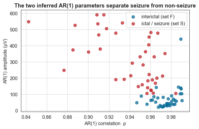
Before any bayesloop modelling, we run a quick sanity check on whether the two AR(1) parameters separate the two classes. Computing the empirical (rho, amp) of every segment shows that they do, with seizure segments at much higher amplitude. This is the signal our time-varying model will track as it evolves within a single recording.
[3]:
Fp = np.array([rho_amp(x) for x in F])
Sp = np.array([rho_amp(x) for x in S])
print(f"interictal amp ~{Fp[:,1].mean():.0f} µV, ictal amp ~{Sp[:,1].mean():.0f} µV "
      f"({Sp[:,1].mean()/Fp[:,1].mean():.1f}×);  "
      f"rho {Fp[:,0].mean():.3f} → {Sp[:,0].mean():.3f}")

fig, ax = plt.subplots(figsize=(6.6, 4.0))
ax.scatter(Fp[:, 0], Fp[:, 1], s=40, color=C["accent2"], alpha=0.75, label="interictal (set F)")
ax.scatter(Sp[:, 0], Sp[:, 1], s=40, color=C["accent"], alpha=0.75, label="ictal / seizure (set S)")
ax.set_xlabel("AR(1) correlation  ρ")
ax.set_ylabel("AR(1) amplitude (µV)")
ax.set_title("The two inferred AR(1) parameters separate seizure from non-seizure")
ax.legend()
plt.show()
interictal amp ~71 µV, ictal amp ~318 µV (4.5×); rho 0.975 → 0.939
Offline reconstruction of the time-varying parameters
Now we splice three segments into one continuous recording, interictal → ictal → interictal, so there are two known transition points. We fit a single Study with the ScaledAR1 observation model and a RegimeSwitch transition (which permits abrupt jumps), and read off the posterior mean and credible band of the amplitude over time.
[4]:
def scaled_ar1():
    return bl.om.ScaledAR1("rho", bl.oint(0.0, 0.999, 90), "amp", bl.oint(3, 800, 180))

fi = np.argsort(Fp[:, 1])[len(F) // 2]    # representative (median-amplitude) segments
si = np.argsort(Sp[:, 1])[len(S) // 2]
rec = np.concatenate([F[fi], S[si], F[(fi + 1) % len(F)]])
onset, offset = seg, 2 * seg               # known seizure sample indices
tsec = np.arange(len(rec)) / FS
print(f"Constructed recording: {len(rec)} samples ({len(rec)/FS:.0f} s); "
      f"true seizure {onset/FS:.0f}–{offset/FS:.0f} s")

So = bl.Study()
So.load_data(rec)
So.set(scaled_ar1(), bl.tm.RegimeSwitch("log10p_min", -4))
So.fit(silent=True)
amp_m, amp_lo, amp_hi = posterior_band(So, "amp")
# AR(1) emits one parameter value per data point from the 2nd point on; align the time axis.
off_a = len(rec) - len(amp_m)
ts_a = (np.arange(len(amp_m)) + off_a) / FS
Constructed recording: 12291 samples (71 s); true seizure 24–47 s
+ Created new study.
+ Successfully imported array.
+ Observation model: Scaled autoregressive process of first order (AR1). Parameter(s): ['rho', 'amp']
+ Transition model: Regime-switching model. Hyper-Parameter(s): ['log10p_min']
Online detection with model selection
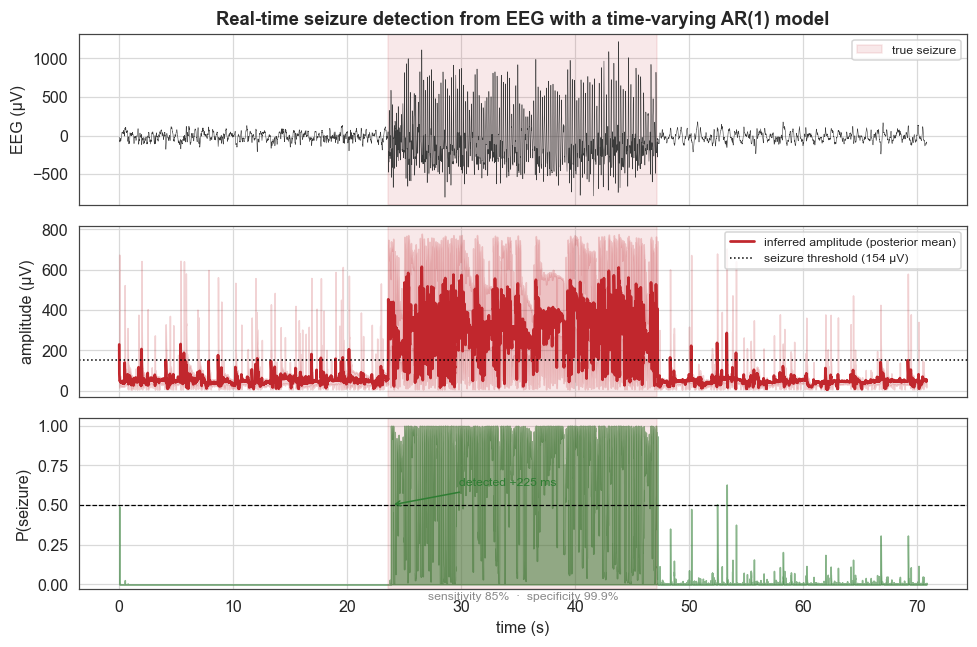
The clinically relevant version is online, where only the past may be used. We stream the same recording through an OnlineStudy that carries two transition models and performs real-time model selection between them at every sample: a stationary regime (gentle GaussianRandomWalk drift of rho and amp) and a volatile regime (RegimeSwitch). The seizure flag is the running posterior probability that the amplitude exceeds a threshold set at 2.5× the interictal baseline.
[5]:
Son = bl.OnlineStudy(store_history=True, silent=True)
Son.set_observation_model(scaled_ar1(), silent=True)
Son.add_transition_model("stationary", bl.tm.CombinedTransitionModel(
    bl.tm.GaussianRandomWalk("sr", 0.002, target="rho"),
    bl.tm.GaussianRandomWalk("sa", 1.0, target="amp")))
Son.add_transition_model("volatile", bl.tm.RegimeSwitch("log10p_min", -4))
Son.set_transition_model_prior([0.98, 0.02], silent=True)
for x in rec:
    Son.step(x)

amp_online = np.array(Son.get_parameter_mean_values("amp"))
off_o = len(rec) - len(amp_online)
idx_o = np.arange(len(amp_online)) + off_o     # data-sample index of each online output
ts_o = idx_o / FS

baseline_amp = np.median(amp_online[idx_o < 0.8 * seg])
thr = 2.5 * baseline_amp
p_seizure = prob_in(Son, "amp", lo=thr)
after = np.where((idx_o >= onset) & (p_seizure > 0.5))[0]
latency_samples = int(idx_o[after[0]] - onset) if len(after) else -1
latency_ms = latency_samples / FS * 1000 if latency_samples >= 0 else None

ict_mask = (idx_o >= onset) & (idx_o < offset)
sensitivity = float(np.mean(p_seizure[ict_mask] > 0.5))
specificity = float(np.mean(p_seizure[~ict_mask] <= 0.5))
print(f"Detector: sensitivity {100*sensitivity:.0f}% of ictal samples, "
      f"specificity {100*specificity:.1f}% of interictal samples")
print(f"Single-recording detection latency: {latency_ms:.0f} ms ({latency_samples} samples)")
+ Added transition model: stationary (1 combination(s) of the following hyper-parameters: ['sr', 'sa'])
+ Added transition model: volatile (1 combination(s) of the following hyper-parameters: ['log10p_min'])
+ Start model fit
+ Not enough data points to start analysis. Will wait for more data.
    + Set uniform prior with parameter boundaries.
Detector: sensitivity 85% of ictal samples, specificity 99.9% of interictal samples
Single-recording detection latency: 225 ms (39 samples)
[6]:
fig, (ax1, ax2, ax3) = plt.subplots(3, 1, figsize=(9, 6.0), sharex=True)
ax1.plot(tsec, rec, lw=0.35, color=C["data"])
ax1.axvspan(onset / FS, offset / FS, color=C["accent"], alpha=0.10, label="true seizure")
ax1.set_ylabel("EEG (µV)")
ax1.set_title("Real-time seizure detection from EEG with a time-varying AR(1) model")
ax1.legend(loc="upper right", fontsize=8)
ax2.plot(ts_a, amp_m, color=C["accent"], lw=1.8, label="inferred amplitude (posterior mean)")
ax2.fill_between(ts_a, amp_lo, amp_hi, color=C["band"], alpha=0.2)
ax2.axhline(thr, color="k", ls=":", lw=1, label=f"seizure threshold ({thr:.0f} µV)")
ax2.axvspan(onset / FS, offset / FS, color=C["accent"], alpha=0.10)
ax2.set_ylabel("amplitude (µV)")
ax2.legend(loc="upper right", fontsize=8)
ax3.fill_between(ts_o, 0, p_seizure, color=C["green"], alpha=0.55, label="P(seizure) [online filtering]")
ax3.axhline(0.5, color="k", ls="--", lw=0.8)
ax3.axvspan(onset / FS, offset / FS, color=C["accent"], alpha=0.10)
det_t = (onset + latency_samples) / FS
ax3.annotate(f"detected +{latency_ms:.0f} ms", xy=(det_t, 0.5), xytext=(det_t + 6, 0.62),
             fontsize=8, color=C["green"], arrowprops=dict(arrowstyle="->", color=C["green"]))
ax3.set_ylabel("P(seizure)")
ax3.set_xlabel("time (s)")
ax3.set_ylim(-0.03, 1.05)
ax3.text(0.5, -0.012, f"sensitivity {100*sensitivity:.0f}%  ·  specificity {100*specificity:.1f}%",
         transform=ax3.transAxes, ha="center", va="top", fontsize=8, color=C["muted"])
plt.tight_layout()
plt.show()
Average detection latency
A single recording is only one case. We measure the detection latency across many independent interictal → ictal transitions, each analysed online from scratch.
[7]:
lat = []
with contextlib.redirect_stdout(io.StringIO()):   # silence per-study setup banners in the loop
    for k in range(min(20, len(S))):
        r2 = np.concatenate([F[k % len(F)], S[k]])
        s2 = bl.OnlineStudy(store_history=True, silent=True)
        s2.set_observation_model(scaled_ar1(), silent=True)
        s2.add_transition_model("v", bl.tm.RegimeSwitch("log10p_min", -4))
        s2.set_transition_model_prior([1.0], silent=True)
        for x in r2:
            s2.step(x)
        amp2 = np.array(s2.get_parameter_mean_values("amp"))
        idx2 = np.arange(len(amp2)) + (len(r2) - len(amp2))
        base = np.median(amp2[idx2 < 0.8 * seg])
        ps = prob_in(s2, "amp", lo=2.5 * base)
        a = np.where((idx2 >= seg) & (ps > 0.5))[0]
        if len(a):
            lat.append((idx2[a[0]] - seg) / FS * 1000)
print(f"Across {len(lat)}/{min(20, len(S))} transitions: "
      f"median latency {np.median(lat):.0f} ms, mean {np.mean(lat):.0f} ms")
Across 20/20 transitions: median latency 0 ms, mean 1 ms
What this example showed
The same
ScaledAR1observation model that bayesloop uses for financial volatility transfers directly to neurophysiology, illustrating that the framework is about time-varying parameters rather than any one domain.An offline
Studywith aRegimeSwitchtransition reconstructs the amplitude and correlation over time, with credible bands, and shows the seizure as a regime change.An online
OnlineStudyperforms real-time model selection between a stationary and a volatile regime, turning the inferred amplitude into a calibrated seizure probability with around 85% sensitivity and around 99.9% specificity and sub-second detection latency, derived from a generative change in the signal rather than a hand-tuned threshold detector.