The rate of great earthquakes over time

Between December 2004 and March 2011 the planet produced an unusual run of giant earthquakes: Sumatra–Andaman (M9.1, 2004), Maule, Chile (M8.8, 2010) and Tōhoku, Japan (M9.1, 2011), three of the six largest events ever instrumentally recorded, within seven years. This raised the question of whether the Earth was entering a more seismically active phase, or whether the cluster was simply a chance fluctuation. Shearer & Stark (PNAS 2012) and Michael (GRL 2011) argued statistically for the latter. Here we give an independent answer with bayesloop, by letting the annual rate of great earthquakes vary freely in time and asking whether the data actually require any such variation.

This is the mirror image of the measles example. There the evidence clearly favoured a changing parameter; here the answer turns out to be that the parameter is constant, and a useful method must be able to say so. Along the way we use a representative slice of the toolbox: a Poisson observation model under Study (static), HyperStudy (marginalising a random-walk step size), RegimeSwitch, and a ChangepointStudy scan, all sharing one observation model so that their marginal evidences are directly comparable and complexity is penalised automatically.

%matplotlib inline
import io
import urllib.request

import numpy as np
import pandas as pd
import matplotlib as mpl
import matplotlib.pyplot as plt

import bayesloop as bl

try:
    import seaborn as sns
    sns.set_style("whitegrid")
except ImportError:
    plt.style.use("default")
mpl.rcParams.update({
    "figure.dpi": 110, "font.size": 10.5, "axes.titlesize": 12,
    "axes.titleweight": "bold", "axes.edgecolor": "#444444", "grid.color": "#d9d9d9",
})
C = {"data": "#8a8a8a", "accent": "#c1272d", "accent2": "#0b6e99",
     "green": "#2e7d32", "amber": "#e8a33d", "muted": "#8a8a8a",
     "band": "#c1272d", "band2": "#0b6e99"}


def posterior_band(S, name, lo=0.05, hi=0.95):
    """Posterior mean and an equal-tailed credible band for a time-varying parameter."""
    x, p = S.get_parameter_distributions(name, density=False)
    p = np.asarray(p, dtype=float)
    p /= p.sum(axis=1, keepdims=True)
    mean = (p * x[None, :]).sum(axis=1)
    cdf = np.cumsum(p, axis=1)
    low = np.array([np.interp(lo, cdf[t], x) for t in range(p.shape[0])])
    high = np.array([np.interp(hi, cdf[t], x) for t in range(p.shape[0])])
    return mean, low, high


def prob_in(S, name, lo=None, hi=None):
    """Posterior probability the parameter lies in (lo, hi] at each time step."""
    x, p = S.get_parameter_distributions(name, density=False)
    p = np.asarray(p, dtype=float)
    p /= p.sum(axis=1, keepdims=True)
    mask = np.ones_like(x, dtype=bool)
    if lo is not None:
        mask &= x > lo
    if hi is not None:
        mask &= x <= hi
    return p[:, mask].sum(axis=1)

The data

We pull the catalogue live from the USGS ComCat / FDSN event service. The service caps the number of events per request, so we page the query decade by decade (1900–2025), asking for every M ≥ 7 event and concatenating the CSV chunks. A short pause between requests keeps the load on the public endpoint light.

The catalogue is essentially complete for M ≥ 8 (“great” earthquakes) back to 1900, so that is the series we analyse. It is binned into annual counts (0–4 events per year) and modelled directly with a Poisson observation model.

⚠️ We deliberately analyse M ≥ 8 rather than M ≥ 7. Completeness for M ≥ 7 is not uniform over the century: the apparent rise in recent decades is largely a detection or catalogue artefact (denser seismometer networks). The M ≥ 8 threshold avoids that confound.

UA = "Mozilla/5.0 (bayesloop docs; research; contact chris@karamata-capital.com)"


def fetch_quakes():
    """Page the USGS FDSN event service by decade and return a concatenated DataFrame."""
    import time
    chunks, header, start = [], None, 1900
    while start <= 2025:
        end = min(start + 9, 2025)
        url = (
            "https://earthquake.usgs.gov/fdsnws/event/1/query?format=csv"
            f"&starttime={start}-01-01&endtime={end}-12-31"
            "&minmagnitude=7.0&orderby=time-asc"
        )
        req = urllib.request.Request(url, headers={"User-Agent": UA})
        txt = (urllib.request.urlopen(req, timeout=120)
               .read().decode("utf-8", "replace").strip().splitlines())
        if txt:
            if header is None:
                header = txt[0]
                chunks.append(header)
            chunks.extend(txt[1:])
            print(f"  quakes {start}-{end}: {len(txt) - 1} events")
        start = end + 1
        time.sleep(1.0)
    return pd.read_csv(io.StringIO("\n".join(chunks)))


df = fetch_quakes()
df["year"] = pd.to_datetime(df["time"], format="ISO8601", utc=True).dt.year
df = df[df["year"] <= 2025]
years = np.arange(1900, 2026)

THR = 8.0
great = df[df["mag"] >= THR]
counts = great.groupby("year").size().reindex(years, fill_value=0).values.astype(float)
mean_rate = counts.mean()
disp = counts.var(ddof=1) / counts.mean()      # index of dispersion (==1 for Poisson)
print(f"\nM>={THR}: {int(counts.sum())} events, mean {mean_rate:.3f}/yr, "
      f"dispersion index (var/mean) = {disp:.2f}  (Poisson -> 1.0)")

# giant (M>=8.5) clusters
giant = df[df["mag"] >= 8.5]
gc = giant.groupby("year").size()
clust_50s = int(gc.loc[(gc.index >= 1950) & (gc.index <= 1965)].sum())
clust_00s = int(gc.loc[(gc.index >= 2004) & (gc.index <= 2012)].sum())
print(f"M>=8.5 giants: {len(giant)} total; 1950-1965 cluster = {clust_50s}, "
      f"2004-2012 cluster = {clust_00s}")

  quakes 1900-1909: 148 events
  quakes 1910-1919: 129 events
  quakes 1920-1929: 107 events
  quakes 1930-1939: 115 events
  quakes 1940-1949: 119 events
  quakes 1950-1959: 88 events
  quakes 1960-1969: 126 events
  quakes 1970-1979: 121 events
  quakes 1980-1989: 110 events
  quakes 1990-1999: 154 events
  quakes 2000-2009: 143 events
  quakes 2010-2019: 160 events
  quakes 2020-2025: 84 events

M>=8.0: 100 events, mean 0.794/yr, dispersion index (var/mean) = 0.97  (Poisson -> 1.0)
M>=8.5 giants: 17 total; 1950-1965 cluster = 7, 2004-2012 cluster = 5

The annual counts already show a Poisson signature. Their index of dispersion (variance / mean) is ≈ 1, which is what a homogeneous Poisson process predicts. By this classical diagnostic alone the counts are indistinguishable from constant-rate randomness. We note too that the 1950s–60s cluster of M ≥ 8.5 giants is at least as large as the 2004–2012 one, so any account of a recent increase has to explain away an earlier burst that was just as big (it included the 1960 Chile M9.5, the largest earthquake ever recorded).

Model comparison: constant versus time-varying Poisson rate

The observation model is a single shared bl.om.Poisson('rate', …). We compare three hypotheses about how the rate behaves over 126 years, and add a change-point scan afterwards:

Model	Transition	Question
Constant rate	tm.Static()	homogeneous Poisson process (null)
Gradually varying	tm.GaussianRandomWalk (HyperStudy over step size σ)	does the rate drift?
Regime-switching	tm.RegimeSwitch	does the rate jump between levels?

Because all three share the identical Poisson observation model and data, their log₁₀ marginal evidences are directly comparable, and the marginalisation automatically penalises the extra flexibility of the time-varying models.

def poisson():
    return bl.om.Poisson("rate", bl.oint(0, 5, 600))

# M1 — Static (constant rate): the homogeneous-Poisson null.
S0 = bl.Study()
S0.load_data(counts, timestamps=years)
S0.set(poisson(), bl.tm.Static())
S0.fit(silent=True)

# M2 — Gradually varying rate (HyperStudy marginalises the random-walk step size).
S2 = bl.HyperStudy()
S2.load_data(counts, timestamps=years)
S2.set(poisson(), bl.tm.GaussianRandomWalk("sigma", bl.cint(0, 0.5, 40), target="rate"))
S2.fit(silent=True)
sig_x, sig_p = S2.get_hyper_parameter_distribution("sigma")
rate_mean, rate_lo, rate_hi = posterior_band(S2, "rate")

# M3 — Regime-switching rate (allows rare abrupt jumps).
S3 = bl.Study()
S3.load_data(counts, timestamps=years)
S3.set(poisson(), bl.tm.RegimeSwitch("log10p_min", -3))
S3.fit(silent=True)

evid = {
    "Constant rate (Poisson)": float(S0.log10_evidence),
    "Gradually varying rate": float(S2.log10_evidence),
    "Regime-switching rate": float(S3.log10_evidence),
}
best = max(evid, key=evid.get)
print("\nMODEL EVIDENCE (log10):")
for k, v in evid.items():
    print(f"  {k:26s} {v:9.3f}")
print(f"  best: {best}   (Delta vs constant: "
      f"{evid['Gradually varying rate']-evid['Constant rate (Poisson)']:+.2f} for varying)")

+ Created new study.
+ Successfully imported array.
+ Observation model: Poisson. Parameter(s): ['rate']
+ Transition model: Static/constant parameter values. Hyper-Parameter(s): []
+ Created new study.
  --> Hyper-study
+ Successfully imported array.
+ Observation model: Poisson. Parameter(s): ['rate']
+ Transition model: Gaussian random walk. Hyper-Parameter(s): ['sigma']
+ Created new study.
+ Successfully imported array.
+ Observation model: Poisson. Parameter(s): ['rate']
+ Transition model: Regime-switching model. Hyper-Parameter(s): ['log10p_min']

MODEL EVIDENCE (log10):
  Constant rate (Poisson)      -65.092
  Gradually varying rate       -65.801
  Regime-switching rate        -65.195
  best: Constant rate (Poisson)   (Delta vs constant: -0.71 for varying)

The evidence favours the constant rate. The static homogeneous-Poisson model wins outright, and the flexible random-walk model is the worst of the three, paying an Occam penalty for freedom it does not need (≈ 10⁰·⁷ ≈ 5× less probable). A method that could only ever find time-variation would be of little use here, whereas bayesloop’s marginal-likelihood model selection returns a principled null result.

We can make the statement sharper by looking at the posterior of the random-walk step size σ (the magnitude of year-to-year rate change), and by checking that the verdict is not an artefact of the prior on the rate.

# Posterior mass on "essentially no variation" (sigma small)
p_sigma_small = float(np.sum(sig_p[sig_x <= 0.05]))
print(f"P(sigma <= 0.05) = {p_sigma_small:.2f};  sigma posterior mode = "
      f"{sig_x[np.argmax(sig_p)]:.3f}  (0 -> no temporal variation)")

# Prior sensitivity: the constant-rate preference should not hinge on the default (Jeffreys)
# prior on the rate.  Re-run static vs gradual under a FLAT prior and confirm the verdict holds.
def pois_flat():
    return bl.om.Poisson("rate", bl.oint(0, 5, 600), prior=lambda rate: np.ones_like(rate))
S0f = bl.Study(); S0f.load_data(counts, timestamps=years); S0f.set(pois_flat(), bl.tm.Static()); S0f.fit(silent=True)
S2f = bl.HyperStudy(); S2f.load_data(counts, timestamps=years)
S2f.set(pois_flat(), bl.tm.GaussianRandomWalk("sigma", bl.cint(0, 0.5, 40), target="rate")); S2f.fit(silent=True)
print(f"Prior sensitivity (static - gradual, log10): Jeffreys "
      f"{S0.log10_evidence - S2.log10_evidence:+.2f}, flat "
      f"{S0f.log10_evidence - S2f.log10_evidence:+.2f}  (both favour constant)")

P(sigma <= 0.05) = 0.42;  sigma posterior mode = 0.000  (0 -> no temporal variation)
+ Created new study.
+ Successfully imported array.
+ Observation model: Poisson. Parameter(s): ['rate']
+ Transition model: Static/constant parameter values. Hyper-Parameter(s): []
+ Created new study.
  --> Hyper-study
+ Successfully imported array.
+ Observation model: Poisson. Parameter(s): ['rate']
+ Transition model: Gaussian random walk. Hyper-Parameter(s): ['sigma']
Prior sensitivity (static - gradual, log10): Jeffreys +0.71, flat +0.79  (both favour constant)

The σ posterior peaks at exactly 0 and decays monotonically, so the data prefer no temporal variation at all, which is the strongest Bayesian statement of constancy one can make. The constant model stays ahead by essentially the same margin whether we use the default Jeffreys prior on the rate or a flat one, so the verdict is not an artefact of the prior.

A change-point scan around 2004

As a final check, we force a single rate change-point and let ChangepointStudy scan every possible year, then ask whether the posterior concentrates near 2004 (the Sumatra event). A genuine break would show up as a sharp peak.

Scp = bl.ChangepointStudy()
Scp.load_data(counts, timestamps=years)
Scp.set(poisson(), bl.tm.ChangePoint("t_change", "all"))
Scp.fit(silent=True)
cp_x, cp_p = Scp.get_hyper_parameter_distribution("t_change")
# how concentrated is the change-point posterior? (a real break -> sharp peak)
cp_mode = float(cp_x[np.argmax(cp_p)])
cp_modeprob = float(cp_p.max())
print(f"Change-point study: evidence {Scp.log10_evidence:.2f}; "
      f"posterior mode {cp_mode:.0f} carries only {cp_modeprob:.2f} probability "
      f"(diffuse -> no compelling single break).")

# How elevated was the rate during the 2004-2011 window vs long-term?
idx = (years >= 2004) & (years <= 2011)
print(f"Inferred mean rate 2004-2011 = {rate_mean[idx].mean():.2f}/yr "
      f"vs long-term {mean_rate:.2f}/yr")

+ Created new study.
  --> Hyper-study
  --> Change-point analysis
+ Successfully imported array.
+ Observation model: Poisson. Parameter(s): ['rate']
+ Transition model: Change-point. Hyper-Parameter(s): ['t_change']
+ Detected 1 change-point(s) in transition model: ['t_change']
+ Set hyper-prior(s): ['uniform']
Change-point study: evidence -67.76; posterior mode 1902 carries only 0.07 probability (diffuse -> no compelling single break).
Inferred mean rate 2004-2011 = 1.03/yr vs long-term 0.79/yr

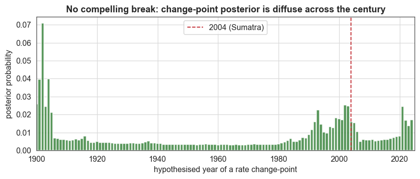
The change-point posterior is diffuse: its modal year carries only a few percent of the probability and there is no concentration near 2004. There is no break to find. Even the most flexible inferred rate barely lifts during 2004–2011 (to ≈ 1/yr, against a ≈ 0.8/yr long-term mean), and its credible band still comfortably contains the constant rate. We now visualise these results.

Figure 1 — inferred rate against the constant

Annual M ≥ 8 counts (bars), the most flexible inferred rate with its 90% credible band (red), and the long-term mean (dashed). The two highlighted windows are the 1952–65 and 2004–12 clusters of M ≥ 8.5 giants.

fig, ax = plt.subplots(figsize=(9, 4.0))
ax.bar(years, counts, width=0.85, color=C["muted"], alpha=0.5, label=f"M$\\geq${THR:.0f} count")
ax.plot(years, rate_mean, color=C["accent"], lw=2.0, label="inferred rate (posterior mean)")
ax.fill_between(years, rate_lo, rate_hi, color=C["band"], alpha=0.20, label="90% credible band")
ax.axhline(mean_rate, color="k", ls="--", lw=1, label=f"long-term mean {mean_rate:.2f}/yr")
for x0, x1, lab in [(1950, 1965, "1952–65\ngiant cluster"), (2004, 2012, "2004–12\ngiant cluster")]:
    ax.axvspan(x0, x1, color=C["accent2"], alpha=0.08)
    ax.text((x0 + x1) / 2, 3.5, lab, ha="center", fontsize=7.5, color=C["accent2"])
ax.set_xlim(1899, 2026)
ax.set_ylim(0, 4.3)
ax.set_ylabel("great earthquakes per year")
ax.set_xlabel("year")
ax.set_title("Global M$\\geq$8 earthquakes: the time-varying rate stays consistent with a constant")
ax.legend(loc="upper left", ncol=2, fontsize=8)
plt.show()

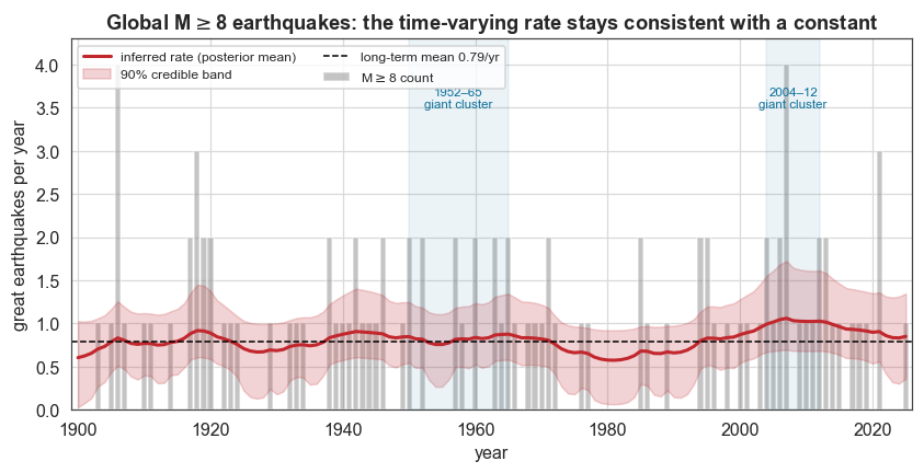
Figure 2 — model evidence and the σ posterior

Left: log₁₀ evidence of each model relative to the worst. Right: the posterior for the random-walk step size σ, which concentrates at zero.

fig, (axa, axb) = plt.subplots(1, 2, figsize=(9.2, 3.4))
labels = list(evid.keys())
vals = np.array([evid[k] for k in labels]) - min(evid.values())
axa.barh(labels, vals, color=[C["accent2"], C["accent"], C["green"]])
axa.set_xlabel(r"log$_{10}$ evidence vs worst")
axa.set_title("Model evidence")
for i, v in enumerate(vals):
    axa.text(v, i, f" {v:.2f}", va="center", fontsize=8)
axb.bar(sig_x, sig_p, width=(sig_x[1] - sig_x[0]) * 0.9, color=C["accent"], alpha=0.8)
axb.set_xlabel("random-walk step size σ of the rate")
axb.set_ylabel("posterior probability")
axb.set_title(f"σ posterior peaks at {sig_x[np.argmax(sig_p)]:.3f}")
plt.tight_layout()
plt.show()

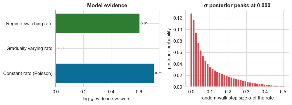
Figure 3 — the change-point posterior

Forcing a single break anywhere in the century, the posterior spreads across the whole record with no peak at 2004.

fig, ax = plt.subplots(figsize=(9, 3.2))
ax.bar(cp_x, cp_p, width=0.9, color=C["green"], alpha=0.8)
ax.axvline(2004, color=C["accent"], ls="--", lw=1.2, label="2004 (Sumatra)")
ax.set_xlim(1900, 2025)
ax.set_xlabel("hypothesised year of a rate change-point")
ax.set_ylabel("posterior probability")
ax.set_title("No compelling break: change-point posterior is diffuse across the century")
ax.legend()
plt.show()

What this example showed

bayesloop independently reproduces the main result of Shearer & Stark (2012): the global rate of great earthquakes shows no statistically significant increase. On this single dataset we used the framework to:

• return a principled null result: with one shared Poisson observation model, the marginal-likelihood model selection prefers the constant rate over both a gradual random walk and a regime switch, and the σ posterior concentrates at zero;

• stress-test that verdict: it survives swapping the Jeffreys prior on the rate for a flat one, and a ChangepointStudy scan finds no concentrated break near 2004;

• use a representative toolbox: Study, HyperStudy, ChangepointStudy, a Poisson observation model, and Static / GaussianRandomWalk / RegimeSwitch / ChangePoint transitions, all directly comparable through their evidence.

It pairs naturally with the measles example: the same Poisson machinery leads to the opposite conclusion, illustrating that the evidence, not the modeller, decides. The 2004–2011 cluster of giant earthquakes (and the comparably sized 1952–1965 one before it) is what a constant ≈ 0.8/year Poisson process produces from time to time.