Weather-adjusted electricity demand and the COVID shock

Utilities weather-normalise electricity demand with a regression on heating-degree-days (HDD): demand = alpha + beta · HDD + noise, where alpha is the weather-independent baseline. Standard practice fits this with constant coefficients, optionally re-estimated per period or in a rolling window. The baseline is not in fact constant; the clearest example is the spring-2020 lockdown, which cut industrial and commercial load. A static fit absorbs that change into its residuals, and a rolling window detects it late and noisily, giving neither a break date nor an uncertainty.

Here we make alpha a time-varying parameter, with beta and the noise inferred jointly. This yields a smooth weather-adjusted baseline with credible bands from a single model that tunes its own smoothness. We then check the result against static and rolling OLS, both on model evidence and on out-of-sample prediction.

%matplotlib inline
import numpy as np
import pandas as pd
import matplotlib as mpl
import matplotlib.pyplot as plt

import statsmodels.api as sm
from statsmodels.regression.rolling import RollingOLS
from scipy.stats import norm

import bayesloop as bl

try:
    import seaborn as sns
    sns.set_style("whitegrid")
except ImportError:
    plt.style.use("default")
mpl.rcParams.update({
    "figure.dpi": 110, "font.size": 10.5, "axes.titlesize": 12,
    "axes.titleweight": "bold", "axes.edgecolor": "#444444", "grid.color": "#d9d9d9",
})
C = {"data": "#3b3b3b", "accent": "#c1272d", "accent2": "#0b6e99",
     "green": "#2e7d32", "amber": "#e8a33d", "muted": "#8a8a8a", "band": "#c1272d"}


def posterior_band(S, name, lo=0.05, hi=0.95):
    """Posterior mean and an equal-tailed credible band for a time-varying parameter."""
    x, p = S.get_parameter_distributions(name, density=False)
    p = np.asarray(p, dtype=float)
    p /= p.sum(axis=1, keepdims=True)
    mean = (p * x[None, :]).sum(axis=1)
    cdf = np.cumsum(p, axis=1)
    low = np.array([np.interp(lo, cdf[t], x) for t in range(p.shape[0])])
    high = np.array([np.interp(hi, cdf[t], x) for t in range(p.shape[0])])
    return mean, low, high

The data

We use German national electricity load (Open Power System Data / ENTSO-E) and Berlin temperature (Open-Meteo), 2015–2020, reduced to small daily series and bundled here. We aggregate to weekly means and form heating-degree-days HDD = max(15 − T, 0). The observation at each week is the pair (demand, HDD).

load = (pd.read_csv("data/energy/de_load_daily.csv", parse_dates=["date"])
        .set_index("date")["load_mw"] / 1000)        # → GW
temp = (pd.read_csv("data/energy/berlin_temp_daily.csv", parse_dates=["date"])
        .set_index("date")["temp_c"])
df = pd.concat([load.rename("gw"), temp.rename("t")], axis=1).dropna().resample("W").mean()
df["hdd"] = np.clip(15.0 - df["t"], 0, None)
weeks = df.index
gw = df["gw"].values
hdd = df["hdd"].values
data = np.column_stack([gw, hdd])
print(f"{len(df)} weeks {weeks.min().date()}..{weeks.max().date()}; "
      f"demand {gw.min():.1f}-{gw.max():.1f} GW")

301 weeks 2015-01-04..2020-10-04; demand 46.5-63.6 GW

Static and rolling OLS

We begin with the standard weather-normalisation regression, both as a single static fit and as a 26-week rolling window. The static slope beta (GW per heating-degree) is the conventional weather-sensitivity coefficient. We hold it fixed in the bayesloop model, exactly as a utility would, and let only the baseline move.

X = sm.add_constant(df["hdd"])
ols = sm.OLS(df["gw"], X).fit()
alpha_static = float(ols.params["const"])
BETA = float(ols.params["hdd"])
resid_static = df["gw"] - ols.predict(X)
roll = RollingOLS(df["gw"], X, window=26).fit()
alpha_roll = roll.params["const"].values
print(f"static OLS: baseline {alpha_static:.1f} GW, beta {BETA:.3f} GW per heating-degree")

static OLS: baseline 52.9 GW, beta 0.463 GW per heating-degree

A time-varying baseline with bayesloop

We write the weather-normalisation regression as a custom om.NumPy observation model with a time-varying baseline alpha and an inferred noise sigma, and let alpha follow a GaussianRandomWalk. A HyperStudy marginalises the random-walk step size, so the time-varying model carries a proper Occam penalty for its flexibility.

def reg(data, alpha, sigma):
    demand, h = data
    mu = alpha + BETA * h
    return np.exp(-(demand - mu) ** 2 / (2 * sigma ** 2)) / np.sqrt(2 * np.pi * sigma ** 2)


def regom():
    return bl.om.NumPy(reg, "alpha", bl.cint(42, 60, 110), "sigma", bl.oint(0.3, 5.0, 50))

S = bl.HyperStudy()
S.load_data(data, timestamps=np.arange(len(df)))
S.set(regom(), bl.tm.GaussianRandomWalk("rw", bl.cint(0, 1.5, 18), target="alpha"))
S.fit(n_jobs=4, silent=True)
alpha_m, alpha_lo, alpha_hi = posterior_band(S, "alpha")
beta_hat = BETA

+ Created new study.
  --> Hyper-study
+ Successfully imported array.
+ Observation model: reg. Parameter(s): ('alpha', 'sigma')
+ Transition model: Gaussian random walk. Hyper-Parameter(s): ['rw']

Comparison by model evidence

This first comparison uses the model evidence. The regression observation model and the fixed beta are the same in both studies; only the alpha-dynamics differ, static versus time-varying. Because the studies share data and likelihood family, their log10_evidence values are directly comparable.

S_static = bl.Study()
S_static.load_data(data, timestamps=np.arange(len(df)))
S_static.set(regom(), bl.tm.Static())
S_static.fit(silent=True)
evid = {"static baseline": float(S_static.log10_evidence),
        "time-varying baseline": float(S.log10_evidence)}
print(f"model evidence (log10): static {evid['static baseline']:.1f} vs "
      f"time-varying {evid['time-varying baseline']:.1f}  "
      f"=> +{S.log10_evidence - S_static.log10_evidence:.1f} for time-varying")

+ Created new study.
+ Successfully imported array.
+ Observation model: reg. Parameter(s): ('alpha', 'sigma')
+ Transition model: Static/constant parameter values. Hyper-Parameter(s): []
model evidence (log10): static -320.6 vs time-varying -305.2  => +15.4 for time-varying

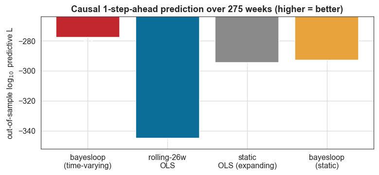
Comparison by out-of-sample prediction

The second comparison is causal out-of-sample prediction. We score the prequential predictive log-likelihood on weeks [B:]: bayesloop via an OnlineStudy (forward-only filtering, no look-ahead), and static and rolling-26-week OLS re-fit on past data only at each step. This is the like-for-like accuracy test that the in-sample residual scatter cannot provide.

B = 26


def online_prequential(tm):
    So = bl.OnlineStudy(silent=True)
    So.set_observation_model(regom(), silent=True)
    So.add_transition_model("m", tm)
    So.set_transition_model_prior([1.0], silent=True)
    le = []
    for row in data:
        So.step(row)
        le.append(So.log_evidence)
    le = np.array(le)
    return float((le[-1] - le[B - 1]) / np.log(10))


def ols_prequential(window=None):
    ll = 0.0
    for t in range(B, len(df)):
        s = slice(0, t) if window is None else slice(max(0, t - window), t)
        Xt = sm.add_constant(df["hdd"].values[s])
        m = sm.OLS(df["gw"].values[s], Xt).fit()
        a, b = m.params
        mu = a + b * df["hdd"].values[t]
        sd = np.sqrt(max(m.mse_resid, 1e-6))
        ll += norm.logpdf(df["gw"].values[t], loc=mu, scale=sd)
    return float(ll / np.log(10))


oos = {
    "bayesloop_time_varying": online_prequential(
        bl.tm.GaussianRandomWalk("rw", bl.cint(0, 1.5, 18), target="alpha")),
    "bayesloop_static": online_prequential(bl.tm.Static()),
    "OLS_static_expanding": ols_prequential(window=None),
    "rolling_OLS_26w": ols_prequential(window=26),
}
print(f"out-of-sample 1-step predictive log10-L over {len(df) - B} weeks:")
for k, v in oos.items():
    print(f"    {k:24s} {v:8.1f}")
print(f"  => bayesloop beats rolling-26w OLS by "
      f"{oos['bayesloop_time_varying'] - oos['rolling_OLS_26w']:+.1f} log10 out-of-sample")

+ Added transition model: m (18 combination(s) of the following hyper-parameters: ['rw'])
+ Start model fit
    + Set uniform prior with parameter boundaries.
+ Added transition model: m (no hyper-parameters)
+ Start model fit
    + Set uniform prior with parameter boundaries.
out-of-sample 1-step predictive log10-L over 275 weeks:
    bayesloop_time_varying     -277.6
    bayesloop_static           -292.9
    OLS_static_expanding       -294.6
    rolling_OLS_26w            -345.1
  => bayesloop beats rolling-26w OLS by +67.5 log10 out-of-sample

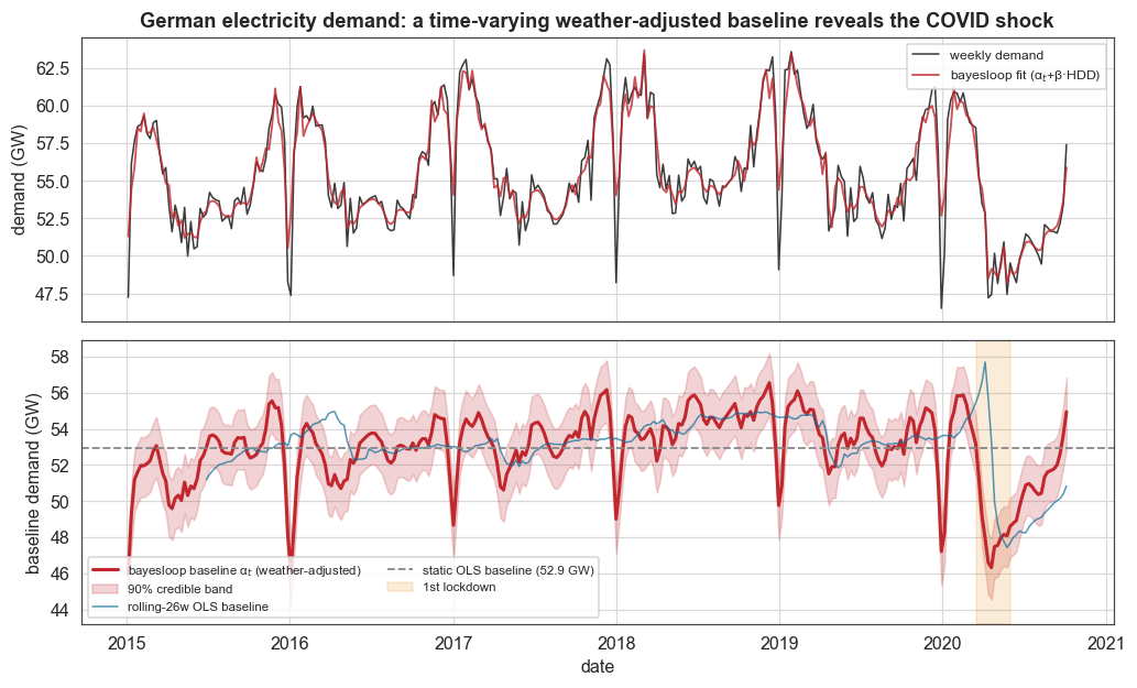
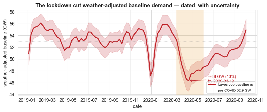
Dating the COVID baseline drop

Finally we read the answer off the inferred baseline: the April-2020 trough versus the same calendar weeks in 2018–2019, which serve as a seasonal control. The time-varying baseline gives a dated drop with uncertainty, whereas the static OLS can only leave it in the residuals.

def spring(yr):
    m = (weeks >= f"{yr}-04-01") & (weeks <= f"{yr}-05-15")
    return alpha_m[m]

ref = np.mean(np.concatenate([spring(2018), spring(2019)]))   # pre-COVID, same season
covid_win = (weeks >= "2020-03-15") & (weeks <= "2020-05-31")
trough = alpha_m[covid_win].min()
trough_week = weeks[covid_win][np.argmin(alpha_m[covid_win])]
pre = ref
static_resid_spring2020 = resid_static[(weeks >= "2020-03-20") & (weeks <= "2020-06-01")].mean()
sigma_hat = float(S.get_parameter_mean_values("sigma")[-1])
print(f"weather-adjusted baseline: pre-COVID {pre:.1f} GW -> {trough_week.date()} "
      f"trough {trough:.1f} GW = -{pre-trough:.1f} GW ({100*(pre-trough)/pre:.1f}%)")
print(f"static-OLS spring-2020 residual: {static_resid_spring2020:.2f} GW (the break it cannot model)")
print(f"in-sample noise: static-OLS residual std {resid_static.std():.2f} GW "
      f"vs bayesloop inferred σ {sigma_hat:.2f} GW")

weather-adjusted baseline: pre-COVID 52.9 GW -> 2020-04-19 trough 46.3 GW = -6.6 GW (12.5%)
static-OLS spring-2020 residual: -5.06 GW (the break it cannot model)
in-sample noise: static-OLS residual std 2.75 GW vs bayesloop inferred σ 1.56 GW

fig, (ax1, ax2) = plt.subplots(2, 1, figsize=(9.4, 5.8), sharex=True)
ax1.plot(weeks, gw, color=C["data"], lw=1.0, label="weekly demand")
ax1.plot(weeks, alpha_m + beta_hat * hdd, color=C["accent"], lw=1.2, alpha=0.8,
         label="bayesloop fit (α$_t$+β·HDD)")
ax1.set_ylabel("demand (GW)")
ax1.set_title("German electricity demand: a time-varying weather-adjusted baseline reveals the COVID shock")
ax1.legend(loc="upper right", fontsize=8)
ax2.plot(weeks, alpha_m, color=C["accent"], lw=2.0, label="bayesloop baseline α$_t$ (weather-adjusted)")
ax2.fill_between(weeks, alpha_lo, alpha_hi, color=C["band"], alpha=0.2, label="90% credible band")
ax2.plot(weeks, alpha_roll, color=C["accent2"], lw=1.0, alpha=0.7, label="rolling-26w OLS baseline")
ax2.axhline(alpha_static, color=C["muted"], ls="--", lw=1.2, label=f"static OLS baseline ({alpha_static:.1f} GW)")
ax2.axvspan(pd.Timestamp("2020-03-15"), pd.Timestamp("2020-06-01"), color=C["amber"], alpha=0.2, label="1st lockdown")
ax2.set_ylabel("baseline demand (GW)")
ax2.set_xlabel("date")
ax2.legend(loc="lower left", fontsize=7.5, ncol=2)
plt.tight_layout()
plt.show()

fig, ax = plt.subplots(figsize=(8.4, 3.6))
mask = weeks >= "2019-01-01"
ax.plot(weeks[mask], alpha_m[mask], color=C["accent"], lw=2.2, label="bayesloop baseline α$_t$")
ax.fill_between(weeks[mask], alpha_lo[mask], alpha_hi[mask], color=C["band"], alpha=0.2)
ax.axhline(pre, color=C["muted"], ls=":", lw=1, label=f"pre-COVID {pre:.1f} GW")
ax.annotate(f"−{pre-trough:.1f} GW ({100*(pre-trough)/pre:.0f}%)\nby {trough_week.date()}",
            xy=(trough_week, trough), xytext=(pd.Timestamp("2020-06-15"), trough - 0.3),
            fontsize=9, color=C["accent"], arrowprops=dict(arrowstyle="->", color=C["accent"]))
ax.axvspan(pd.Timestamp("2020-03-15"), pd.Timestamp("2020-06-01"), color=C["amber"], alpha=0.2)
ax.set_ylabel("weather-adjusted baseline (GW)")
ax.set_xlabel("date")
ax.set_title("The lockdown cut weather-adjusted baseline demand — dated, with uncertainty")
ax.legend(loc="lower right", fontsize=8)
plt.tight_layout()
plt.show()

fig, ax = plt.subplots(figsize=(7.2, 3.4))
lab = ["bayesloop\n(time-varying)", "rolling-26w\nOLS", "static\nOLS (expanding)", "bayesloop\n(static)"]
key = ["bayesloop_time_varying", "rolling_OLS_26w", "OLS_static_expanding", "bayesloop_static"]
vv = [oos[k] for k in key]
bars = ax.bar(lab, vv, color=[C["accent"], C["accent2"], C["muted"], C["amber"]])
ax.set_ylabel(r"out-of-sample $\log_{10}$ predictive L")
ax.set_title(f"Causal 1-step-ahead prediction over {len(df) - B} weeks (higher = better)")
ax.set_ylim(min(vv) * 1.02, max(vv) * 0.95)
for b, v in zip(bars, vv):
    ax.text(b.get_x() + b.get_width() / 2, v, f"{v:.0f}", ha="center", va="top", fontsize=8, color="white")
plt.tight_layout()
plt.show()

What this example showed

On weekly German electricity demand we used bayesloop to:

• turn a textbook weather-normalisation regression into a time-varying-coefficient model with a custom om.NumPy observation model, so that the baseline can move, with beta and the noise inferred jointly and the random-walk smoothness tuned by a HyperStudy;

• compare it against the standard models on the same terms: it reaches a higher model evidence than a static baseline, and gives better out-of-sample one-step prediction than both static and rolling-window OLS;

• recover information the standard workflow cannot, namely a dated COVID baseline drop (≈ −6.6 GW, ~13%) with a credible band, rather than an unexplained lump in the residuals.