Measles in the United States: abrupt break or gradual decline

This example applies bayesloop to a question from epidemiology. Measles is one of the great success stories of public health: a vaccine was licensed in 1963 and the United States declared the disease eliminated in 2000. The textbook narrative is a clean before/after story, but it is not obvious whether the vaccine’s epidemiological signature was really an abrupt break or a gradual multi-year decline as coverage accumulated. A related question is whether the transition can be dated from the data alone, without assuming when it happened.

These are questions bayesloop is built for. Rather than fitting one static model, we let the transmission level vary in time and use the marginal likelihood (model evidence) as an objective, complexity-penalised score to ask the data which kind of variation it prefers. In the course of the analysis we use a good part of the toolbox: Study, HyperStudy and ChangepointStudy; the Gaussian and custom NumPy observation models; and the Static, GaussianRandomWalk, AlphaStableRandomWalk, ChangePoint, CombinedTransitionModel and RegimeSwitch transition models.

import io
import urllib.request

import numpy as np
import pandas as pd
import matplotlib as mpl
import matplotlib.pyplot as plt

import bayesloop as bl

# A consistent, publication-leaning style for the figures below.
try:
    import seaborn as sns
    sns.set_style("whitegrid")
except ImportError:
    plt.style.use("default")
mpl.rcParams.update({
    "figure.dpi": 110, "font.size": 10.5, "axes.titlesize": 12,
    "axes.titleweight": "bold", "axes.edgecolor": "#444444", "grid.color": "#d9d9d9",
})
C = {"data": "#8a8a8a", "accent": "#c1272d", "accent2": "#0b6e99", "green": "#2e7d32"}


# Two small helpers to turn a fitted study into a posterior mean and credible band for
# a time-varying parameter. (bayesloop also has built-in plotting via ``S.plot``; these
# give us a bit more control over the figures.)
def posterior_band(S, name, lo=0.05, hi=0.95):
    """Posterior mean and an equal-tailed credible band for a time-varying parameter."""
    x, p = S.get_parameter_distributions(name, density=False)
    p = np.asarray(p, dtype=float)
    p /= p.sum(axis=1, keepdims=True)
    mean = (p * x[None, :]).sum(axis=1)
    cdf = np.cumsum(p, axis=1)
    low = np.array([np.interp(lo, cdf[t], x) for t in range(p.shape[0])])
    high = np.array([np.interp(hi, cdf[t], x) for t in range(p.shape[0])])
    return mean, low, high


def prob_above(S, name, threshold):
    """Posterior probability that the parameter exceeds ``threshold`` at each time step."""
    x, p = S.get_parameter_distributions(name, density=False)
    p = np.asarray(p, dtype=float)
    p /= p.sum(axis=1, keepdims=True)
    return p[:, x > threshold].sum(axis=1)

The data

We use US national annual measles case counts from Our World in Data (compiled from US CDC notifiable-disease reports / Project Tycho). The series is contiguous from 1938 to 2025 and spans almost five orders of magnitude, from nearly a million cases a year before the vaccine to a few dozen after elimination. Because of this large dynamic range we model log₁₀(cases) with a Gaussian observation model (standard practice for incidence data); we return to the natural count scale for the modern post-elimination era at the end.

url = "https://ourworldindata.org/grapher/number-of-measles-cases.csv?csvType=full"
req = urllib.request.Request(url, headers={"User-Agent": "Mozilla/5.0 (bayesloop docs)"})
df = pd.read_csv(io.BytesIO(urllib.request.urlopen(req, timeout=90).read()))

col = [c for c in df.columns if "measles" in c.lower() and "Annot" not in c][0]
us = (df[df["Entity"] == "United States"][["Year", col]]
      .rename(columns={col: "cases"}).sort_values("Year").reset_index(drop=True))
us = us[us["Year"] <= 2025]
full = us[us["Year"] >= 1938].reset_index(drop=True)

years = full["Year"].values.astype(float)
cases = full["cases"].values.astype(float)
logcases = np.log10(cases)
print(f"Full record: {int(years.min())}-{int(years.max())} "
      f"({len(years)} years), cases {int(cases.min())}-{int(cases.max())}")

Full record: 1938-2025 (88 years), cases 13-894134

A time-varying transmission level

Our observation model treats each year’s log-incidence as Gaussian with a time-varying mean (the transmission level) and a free standard deviation, which absorbs the strong biennial epidemic cycles of the pre-vaccine era:

bl.om.Gaussian("mean", ..., "std", ...)

For the dynamics of that mean we start with a GaussianRandomWalk, so the level is allowed to drift smoothly from year to year, and wrap it in a HyperStudy, which marginalises over the unknown magnitude (sigma) of that drift.

def gaussian_obs():
    return bl.om.Gaussian("mean", bl.cint(0.5, 6.5, 240),
                          "std", bl.oint(0.03, 1.2, 90))

Sg = bl.HyperStudy()
Sg.load_data(logcases, timestamps=years)
Sg.set(gaussian_obs(),
       bl.tm.GaussianRandomWalk("sigma", bl.cint(0, 0.6, 30), target="mean"))
Sg.fit()
evidence_gradual = float(Sg.log10_evidence)

+ Created new study.
  --> Hyper-study
+ Successfully imported array.
+ Observation model: Gaussian observations. Parameter(s): ['mean', 'std']
+ Transition model: Gaussian random walk. Hyper-Parameter(s): ['sigma']
+ Set hyper-prior(s): ['uniform']
+ Started new fit.
    + 30 analyses to run.
    + Cached observation likelihoods (14.5 MiB).
    + Computed average posterior sequence
    + Computed hyper-parameter distribution
    + Log10-evidence of average model: -22.16384
    + Computed local evidence of average model
    + Computed mean parameter values.
+ Finished fit.

Left free to maximise evidence, the random walk picks a fairly large step size. It has to, in order to follow the steep 1960s decline, and a single global step size cannot also be small in the flat plateaus. As a side-effect, the evidence-optimal fit tracks year-to-year epidemic variation rather than smoothing it. For visualising the secular trend we therefore also fit a deliberately regularised version with a small, fixed step. The model-selection conclusion below turns out to be robust to this choice.

Ssm = bl.Study()
Ssm.load_data(logcases, timestamps=years)
Ssm.set(gaussian_obs(), bl.tm.GaussianRandomWalk("sigma", 0.10, target="mean"))
Ssm.fit(silent=True)
mean_sm, lo_sm, hi_sm = posterior_band(Ssm, "mean")

fig, ax = plt.subplots(figsize=(9, 4.2))
ax.bar(years, cases, width=0.8, color=C["data"], alpha=0.45, label="reported cases")
ax.plot(years, 10 ** mean_sm, color=C["accent"], lw=2.2,
        label="inferred transmission trend (smoothed)")
ax.fill_between(years, 10 ** lo_sm, 10 ** hi_sm, color=C["accent"], alpha=0.20,
                label="90% credible band")
ax.set_yscale("log")
ax.set_ylim(8, 2e6)
ax.set_xlim(1937, 2026)
for yr, lab in [(1963, "vaccine\nlicensed 1963"), (1989, "1989–91\nresurgence"),
                (2000, "elimination\ndeclared 2000")]:
    ax.axvline(yr, color=C["accent2"], ls="--", lw=1, alpha=0.6)
    ax.text(yr + 0.5, 1.1e6, lab, fontsize=7.5, color=C["accent2"], va="top")
ax.set_ylabel("measles cases per year")
ax.set_xlabel("year")
ax.set_title("US measles: a time-varying transmission level inferred by bayesloop")
ax.legend(loc="lower left", ncol=2)
plt.show()

+ Created new study.
+ Successfully imported array.
+ Observation model: Gaussian observations. Parameter(s): ['mean', 'std']
+ Transition model: Gaussian random walk. Hyper-Parameter(s): ['sigma']

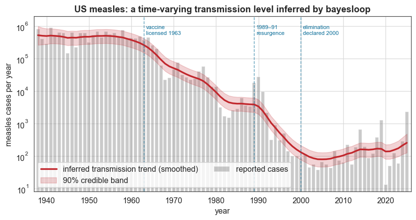
The inferred trend reproduces the modern history of US measles: the pre-vaccine plateau near 5 × 10⁵ cases/year, the post-1963 collapse, the 1989–91 resurgence (resolved as a temporary bump), the drive to elimination, and the recent resurgence.

Letting the evidence choose between abrupt and gradual change

The picture above assumes gradual drift. Whether the data actually prefer that over the alternatives is a question we can answer directly. Because every model below shares the identical observation model and data, their log₁₀ marginal likelihoods (S.log10_evidence) are directly comparable. We compare four hypotheses:

Hypothesis	Transition model
Static (null)	tm.Static()
Abrupt change-point	tm.ChangePoint("t_change", "all")
Gradual random walk	tm.GaussianRandomWalk (the HyperStudy above)
Change-point + drift	CombinedTransitionModel(ChangePoint, GaussianRandomWalk)

# M0 — Static (constant level): the null hypothesis.
S0 = bl.Study()
S0.load_data(logcases, timestamps=years)
S0.set(gaussian_obs(), bl.tm.Static())
S0.fit(silent=True)

# M1 — a single abrupt change-point. ChangepointStudy scans *every* possible break year.
S1 = bl.ChangepointStudy()
S1.load_data(logcases, timestamps=years)
S1.set(gaussian_obs(), bl.tm.ChangePoint("t_change", "all"))
S1.fit(silent=True)
cp_x, cp_p = S1.get_hyper_parameter_distribution("t_change")
cp_mode = float(cp_x[np.argmax(cp_p)])
order = np.argsort(cp_p)[::-1]
cred = np.sort(cp_x[order[:np.searchsorted(np.cumsum(cp_p[order]), 0.90) + 1]])

# M3 — an abrupt break superimposed on gradual drift.
S3 = bl.ChangepointStudy()
S3.load_data(logcases, timestamps=years)
S3.set(gaussian_obs(),
       bl.tm.CombinedTransitionModel(
           bl.tm.ChangePoint("t_change", "all"),
           bl.tm.GaussianRandomWalk("sigma", 0.15, target="mean")))
S3.fit(silent=True)

evidence = {
    "Static (constant)": float(S0.log10_evidence),
    "Abrupt change-point": float(S1.log10_evidence),
    "Gradual random walk": evidence_gradual,
    "Change-point + drift": float(S3.log10_evidence),
}
best = max(evidence, key=evidence.get)
print("Model evidence (log10, higher is better):")
for k, v in evidence.items():
    print(f"  {k:24s} {v:9.2f}")
print(f"  --> best: {best}")
print(f"Change-point mode: {cp_mode:.0f} (90% credible {cred.min():.0f}-{cred.max():.0f})")

+ Created new study.
+ Successfully imported array.
+ Observation model: Gaussian observations. Parameter(s): ['mean', 'std']
+ Transition model: Static/constant parameter values. Hyper-Parameter(s): []
+ Created new study.
  --> Hyper-study
  --> Change-point analysis
+ Successfully imported array.
+ Observation model: Gaussian observations. Parameter(s): ['mean', 'std']
+ Transition model: Change-point. Hyper-Parameter(s): ['t_change']
+ Detected 1 change-point(s) in transition model: ['t_change']
+ Set hyper-prior(s): ['uniform']
+ Created new study.
  --> Hyper-study
  --> Change-point analysis
+ Successfully imported array.
+ Observation model: Gaussian observations. Parameter(s): ['mean', 'std']
+ Transition model: Combined transition model. Hyper-Parameter(s): ['t_change', 'sigma']
+ Detected 1 change-point(s) in transition model: ['t_change']
+ Set hyper-prior(s): ['uniform', 'uniform']
Model evidence (log10, higher is better):
  Static (constant)           -78.56
  Abrupt change-point         -47.12
  Gradual random walk         -22.16
  Change-point + drift        -25.16
  --> best: Gradual random walk
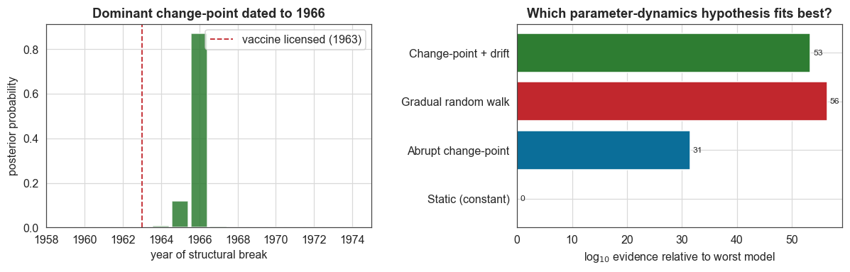
Change-point mode: 1966 (90% credible 1965-1966)

The gradual random walk wins by a wide margin. It is many orders of magnitude more probable than a single abrupt change-point, and adding a change-point on top of the drift makes the model worse, as the Occam penalty for the extra parameter is not repaid. The scientific reading is clear and non-trivial: the vaccine’s epidemiological footprint is not a single clean break but a sustained, multi-decade decline as coverage ratcheted up.

When we nonetheless force a single change-point, the posterior dates the dominant break to within a couple of years of the 1963 licensing, the lag expected for mass uptake, and gives a credible interval for it, which a fixed before/after split never could.

fig, (axL, axR) = plt.subplots(1, 2, figsize=(11, 3.6))

# change-point posterior
axL.bar(cp_x, cp_p, width=0.85, color=C["green"], alpha=0.85)
axL.set_xlim(1958, 1975)
axL.axvline(1963, color=C["accent"], ls="--", lw=1.2, label="vaccine licensed (1963)")
axL.set_xlabel("year of structural break")
axL.set_ylabel("posterior probability")
axL.set_title(f"Dominant change-point dated to {cp_mode:.0f}")
axL.legend()

# evidence comparison
labels = list(evidence)
vals = np.array([evidence[k] for k in labels])
vals_rel = vals - vals.min()
bars = axR.barh(labels, vals_rel, color=[C["data"], C["accent2"], C["accent"], C["green"]])
axR.set_xlabel(r"log$_{10}$ evidence relative to worst model")
axR.set_title("Which parameter-dynamics hypothesis fits best?")
for b, v in zip(bars, vals_rel):
    axR.text(v + max(vals_rel) * 0.01, b.get_y() + b.get_height() / 2,
             f"{v:.0f}", va="center", fontsize=8)
plt.tight_layout()
plt.show()

Robustness of the gradual model

One concern is whether the gradual model won only because it was allowed to over-fit. We check this by comparing the heavily regularised smoothed fit (small fixed step) against the alternatives, and by trying a heavier-tailed AlphaStableRandomWalk that permits occasional large jumps rather than uniform Gaussian steps (a 2-D HyperStudy over the scale c and the tail index alpha).

Sas = bl.HyperStudy()
Sas.load_data(logcases, timestamps=years)
Sas.set(gaussian_obs(),
        bl.tm.AlphaStableRandomWalk("c", bl.cint(0.01, 0.5, 10),
                                    "alpha", bl.cint(1.1, 2.0, 8), target="mean"))
Sas.fit(silent=True, n_jobs=4)
a_x, a_p = Sas.get_hyper_parameter_distribution("alpha")
print(f"Regularised smooth fit (sigma=0.10): log10 evidence = {Ssm.log10_evidence:7.2f}")
print(f"Alpha-stable random walk:            log10 evidence = {Sas.log10_evidence:7.2f}"
      f"  (tail index alpha mode = {a_x[np.argmax(a_p)]:.2f})")

+ Created new study.
  --> Hyper-study
+ Successfully imported array.
+ Observation model: Gaussian observations. Parameter(s): ['mean', 'std']
+ Transition model: Alpha-stable random walk. Hyper-Parameter(s): ['c', 'alpha']
Regularised smooth fit (sigma=0.10): log10 evidence =  -29.17
Alpha-stable random walk:            log10 evidence =  -19.84  (tail index alpha mode = 1.74)

Even the regularised fit comfortably beats the single change-point, so the win comes from the sustained, multi-decade nature of the decline rather than from over-fitting. The alpha-stable model fits best of all, with a tail index alpha well below 2, indicating that the decline is best described by occasional large jumps on top of gentle drift.

We can also quote a model-free magnitude straight from the raw series:

pre = float(np.mean(cases[(years >= 1938) & (years <= 1962)]))
lowmask = (years >= 1980) & (years <= 1985)
trough = float(cases[lowmask].min())
trough_year = float(years[lowmask][np.argmin(cases[lowmask])])
print(f"Pre-vaccine mean (1938-1962): {pre:,.0f} cases/yr")
print(f"Early-1980s trough ({trough_year:.0f}): {trough:,.0f} cases")
print(f"=> {pre/trough:,.0f}-fold reduction")

Pre-vaccine mean (1938-1962): 532,633 cases/yr
Early-1980s trough (1983): 1,497 cases
=> 356-fold reduction

The post-elimination era: a custom Poisson observation model

After elimination the counts are small enough (tens to a couple thousand) to model directly as Poisson rather than on the log scale. This is also an occasion to show bayesloop’s extensibility. Its built-in Poisson evaluates the pmf directly, which overflows for counts above about 170, so we supply a numerically stable log-space Poisson as a one-line bl.om.NumPy custom model. We pair it with a RegimeSwitch transition, which lets the rate jump abruptly and is well suited to detecting outbreaks against the near-zero eliminated baseline.

from scipy.special import gammaln

def poisson_stable(data, rate):
    k = float(data)
    return np.exp(k * np.log(rate) - rate - gammaln(k + 1.0))

modern = us[(us["Year"] >= 1998) & (us["Year"] <= 2025)].reset_index(drop=True)
myears = modern["Year"].values.astype(float)
mcases = modern["cases"].values.astype(float)

Sp = bl.Study()
Sp.load_data(mcases, timestamps=myears)
Sp.set(bl.om.NumPy(poisson_stable, "rate", bl.oint(0, 3000, 1500)),
       bl.tm.RegimeSwitch("log10p_min", -4))
Sp.fit()

rate_mean, rate_lo, rate_hi = posterior_band(Sp, "rate")
baseline = float(np.median(rate_mean[(myears >= 1998) & (myears <= 2017)]))
p_outbreak = prob_above(Sp, "rate", 5 * baseline)   # P(rate > 5x baseline)
for y in (2019, 2025):
    print(f"  {y}: {int(mcases[myears == y][0]):>5d} cases, "
          f"P(rate > 5x baseline) = {p_outbreak[myears == y][0]:.2f}")

+ Created new study.
+ Successfully imported array.
+ Observation model: poisson_stable. Parameter(s): ('rate',)
+ Transition model: Regime-switching model. Hyper-Parameter(s): ['log10p_min']
+ Started new fit:
    + Formatted data.
    + Cached observation likelihoods (0.3 MiB).
    + Set uniform prior with parameter boundaries.
    + Finished forward pass.
    + Log10-evidence: -93.44755
    + Finished backward pass.
    + Computed mean parameter values.
  2019:  1274 cases, P(rate > 5x baseline) = 1.00
  2025:  2288 cases, P(rate > 5x baseline) = 1.00

fig, (ax1, ax2) = plt.subplots(2, 1, figsize=(9, 4.6), sharex=True,
                               gridspec_kw={"height_ratios": [2, 1]})
ax1.bar(myears, mcases, width=0.7, color=C["data"], alpha=0.5, label="reported cases")
ax1.plot(myears, rate_mean, color=C["accent"], lw=2, label="inferred Poisson rate")
ax1.fill_between(myears, rate_lo, rate_hi, color=C["accent"], alpha=0.2)
ax1.axhline(baseline, color=C["accent2"], ls=":", lw=1, label=f"baseline ~{baseline:.0f}/yr")
ax1.set_ylabel("cases / yr")
ax1.set_title("Post-elimination era: a regime-switching Poisson rate detects outbreaks")
ax1.legend(loc="upper left", fontsize=8)
ax2.bar(myears, p_outbreak, width=0.7, color=C["green"], alpha=0.7)
ax2.set_ylabel("P(rate > 5×base)")
ax2.set_xlabel("year")
ax2.set_ylim(0, 1)
plt.tight_layout()
plt.show()

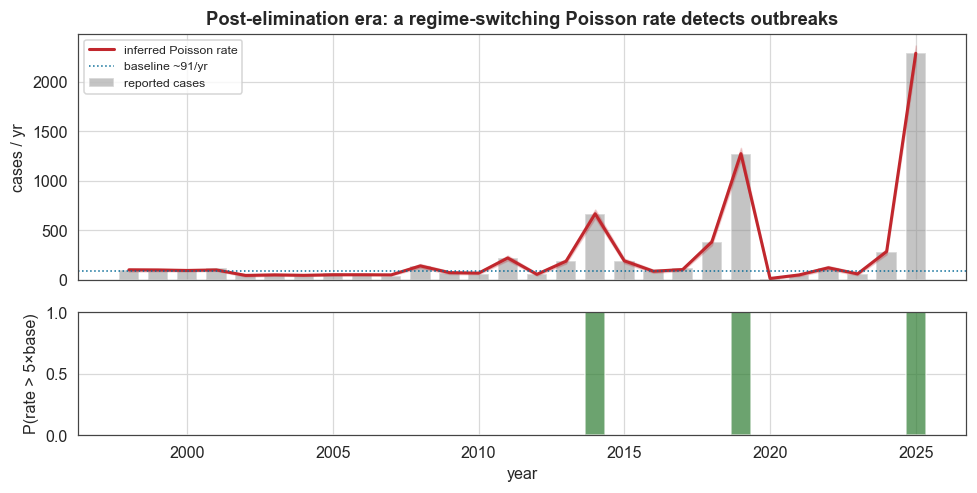
The regime-switching Poisson flags the 2019 and 2025 outbreaks at posterior probability ≈ 1.0 against the eliminated baseline.

What this example showed

On a single dataset we used bayesloop to:

• answer a scientific question with model evidence: the choice between abrupt and gradual change is settled quantitatively, and the answer (gradual) is the less obvious one;

• recover a dated transition with a credible interval, without telling the model when the vaccine arrived;

• exercise the toolbox end-to-end, using Study, HyperStudy and ChangepointStudy, the Gaussian and custom NumPy observation models, and a range of transition models including a custom numerically-stable Poisson and a regime switch.

Every number cross-checks against the published epidemiological record: a ~1966 dominant transition, the early-1980s trough, the ~356-fold drop, the 1989–91 resurgence, and the 2019/2025 outbreaks.