Online study

OnlineStudy performs sequential inference: new observations are incorporated one at a time with step, and the current posterior becomes the prior for the next update. This is useful when data arrive from a stream and the complete time series is not available upfront.

The example below reuses the coal mining disaster data, but feeds the observations to the model one after another. We compare a static rate model against a dynamic rate model while storing the full history for plotting.

%matplotlib inline
import matplotlib.pyplot as plt
plt.style.use('seaborn-v0_8-whitegrid')  # plot styling

import bayesloop as bl

source = bl.Study(silent=True)
source.load_example_data(silent=True)
data = source.raw_data
years = source.raw_timestamps

S = bl.OnlineStudy(store_history=True, silent=True)

L = bl.om.Poisson('accident_rate', bl.oint(0, 6, 300))
S.set_observation_model(L, silent=True)

S.add_transition_model('static', bl.tm.Static())
S.add_transition_model('dynamic', bl.tm.GaussianRandomWalk('sigma', [0.1, 0.3], target='accident_rate'))
S.set_transition_model_prior([0.5, 0.5], silent=True)

for value in data:
    S.step(value)

+ Added transition model: static (no hyper-parameters)
+ Added transition model: dynamic (2 combination(s) of the following hyper-parameters: ['sigma'])
+ Start model fit
    + Set prior (function): jeffreys. Values have been re-normalized.

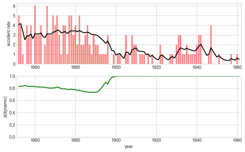
The stored history can be queried just like in a retrospective study. Here we plot the posterior mean of the accident rate and the accumulated probability of the dynamic transition model.

rate_mean = S.get_parameter_mean_values('accident_rate')
dynamic_probability = S.get_transition_model_probabilities('dynamic')

plt.figure(figsize=(8, 5))

plt.subplot(211)
plt.bar(years, data, align='center', facecolor='r', alpha=.45)
plt.plot(years, rate_mean, color='k', lw=2)
plt.xlim([1851, 1962])
plt.ylabel('accident rate')

plt.subplot(212)
plt.plot(years, dynamic_probability, color='g', lw=2)
plt.xlim([1851, 1962])
plt.ylim([0, 1])
plt.xlabel('year')
plt.ylabel('p(dynamic)')

plt.tight_layout();

For a larger OnlineStudy use case with multiple transition models and hyperparameter grids, see the stock market fluctuations example.