Hyper-study

The time series models built with the help of bayesloop are called hierarchical models, since the parameters of the observation model are in turn controlled by hyper-parameters that are possibly included in the transition model. In the previous section, we optimized two hyper-parameters of a serially combined transition model: the slope of the decrease in coal mining disasters from 1885 to 1895, and the magnitude of the fluctuations afterwards. While the optimization routine yields the most probable values of these hyper-parameters, one might also be interested in the uncertainty tied to these “optimal” values. bayesloop therefore provides the HyperStudy class that allows to compute the full distribution of hyper-parameters by defining a discrete grid of hyper-parameter values.

While the HyperStudy instance can be configured just like a standard Study instance, one may supply not only single hyper-parameter values, but also lists/arrays of values (Note: It will fall back to the standard fit method if only one combination of hyper-parameter values is supplied). Here, we test a range on hyper-parameter values by supplying regularly spaced hyper-parameter values using the cint function (one can of course also use similar functions like numpy.linspace). In the example below, we return to the serial transition model used here and compute a two-dimensional distribution of the two hyper-parameters slope (20 steps from -0.4 to 0.0) and sigma (20 steps from 0.0 to 0.8).

After running the fit-method for all value-tuples of the hyper-grid, the model evidence values of the individual fits are used as weights to compute weighted average parameter distributions. These average parameter distributions allow to assess the temporal evolution of the model parameters, explicitly considering the uncertainty of the hyper-parameters. However, in case one is only interested in the hyper-parameter distribution, setting the keyword-argument evidenceOnly=True of the fit method shortens the computation time but skips the evaluation of parameter distributions.

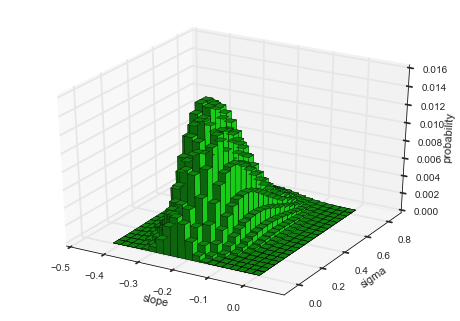
Finally, bayesloop provides several methods to plot the results of the hyper-study. To display the joint distribution of two hyper-parameters, choose getJointHyperParameterDistribution (or shorter: getJHPD). The method automatically computes the marginal distribution for the two specified hyper-parameters and returns three arrays, two for the hyper-parameters values and one with the corresponding probability values. Here, the first argument represents a list of two hyper-parameter names. If the keyword-argument plot=True is set, a visualization is created using the bar3d function from the mpl_toolkits.mplot3d module.

%matplotlib inline
import matplotlib.pyplot as plt # plotting
import seaborn as sns           # nicer plots
sns.set_style('whitegrid')      # plot styling

import numpy as np
import bayesloop as bl

S = bl.HyperStudy()
S.loadExampleData()

L = bl.om.Poisson('accident_rate', bl.oint(0, 6, 1000))

T = bl.tm.SerialTransitionModel(bl.tm.Static(),
                                bl.tm.BreakPoint('t_1', 1885),
                                bl.tm.Deterministic(lambda t, slope=bl.cint(-0.4, 0, 20): slope*t,
                                                    target='accident_rate'),
                                bl.tm.BreakPoint('t_2', 1895),
                                bl.tm.GaussianRandomWalk('sigma', bl.cint(0, 0.8, 20),
                                                         target='accident_rate'))
S.set(L, T)

S.fit()
S.getJointHyperParameterDistribution(['slope', 'sigma'], plot=True, color=[0.1, 0.8, 0.1])

plt.xlim([-0.5, 0.1])
plt.ylim([-0.1, 0.9]);

+ Created new study.
  --> Hyper-study
+ Successfully imported example data.
+ Observation model: Poisson. Parameter(s): ['accident_rate']
+ Transition model: Serial transition model. Hyper-Parameter(s): ['slope', 'sigma', 't_1', 't_2']
+ Set hyper-prior(s): ['uniform', 'uniform', 'uniform', 'uniform']
+ Started new fit.
    + 400 analyses to run.

    + Computed average posterior sequence
    + Computed hyper-parameter distribution
    + Log10-evidence of average model: -73.47969
    + Computed local evidence of average model
    + Computed mean parameter values.
+ Finished fit.

It is important to note here, that the evidence value of \(\approx 10^{-73.5}\) is smaller compared to the value of \(\approx 10^{-72.7}\) obtained in a previous analysis here. There, we optimized the hyper-parameter values and assumed that these optimal values are not subject to uncertainty, therefore over-estimating the model evidence. In contrast, the hyper-study explicitly considers the uncertainty tied to the hyper-parameter values.

While the joint distribution of two hyper-parameters may uncover possible correlations between the two quantities, the 3D plot is often difficult to integrate into existing figures. To plot the marginal distribution of a single hyper-parameter in a simple 2D histogram/bar plot, use the plot method, just as for the parameters of the observation model:

plt.figure(figsize=(16,4))
plt.subplot(121)
S.plot('slope', color='g', alpha=.8);

plt.subplot(122)
S.plot('sigma', color='g', alpha=.8);

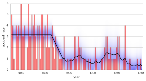
Finally, the temporal evolution of the model parameter may be displayed using, again, the plot method:

plt.figure(figsize=(8, 4))
plt.bar(S.rawTimestamps, S.rawData, align='center', facecolor='r', alpha=.5)
S.plot('accident_rate')
plt.xlim([1851, 1962])
plt.xlabel('year');

In principle, a HyperStudy could also be used to test different time stamps for change- and break-points. However, in a transition model with several change- or break-points, the correct order has to be maintained. Since a HyperStudy fits all possible combinations of hyper-parameter values, we need another type of study that takes care of the correct order of change-/break-points, the ChangepointStudy class. It is introduced in the next tutorial.